
Publications
My most recent papers (published in July and November 2022 - the July paper was featured in ApJ Year in Review 2022 as one of the most popular papers of 2022), were on constraining the accretion rate distribution (also known as Eddington ratio distribution function; ERDF) of obscured AGN using Swift-BAT and BASS DR2 data. This is the first directly observationally constrained ERDF calculated using an X-ray-selected sample. We find that the intrinsic ERDF of obscured (Type 2) and unobscured (Type 1) AGN are significantly different from each other. In the November 2022 letter, we discuss the difference in ERDFs of AGN categorized by broad/narrow lines and X-ray-based obscuring column densities (e.g., log NH). The physical implications of all our findings are also discussed in this paper.
Click to see a full ADS record of refereed publications.
Here you can find the ADS record of my first-author publications.
RESEARCH SUMMARIES
Online Colloquium
A colloquium that I presented at NASA’s Goddard Space Flight Center (October 2021) summarizes the most exciting results from my work.
Projects
A publicly available X-ray Stacking Software StackFast

HEAD Meeting Poster, March 2022
X-ray stacking software STACKFAST (publicly available at this link) works in two steps: (1) extracting photons and exposure information from the NuSTAR and Chandra data sets for every object in a master source catalog, and (2) allowing the user to coadd the emission from any subset within the master catalog. Of these, only step (1) is computationally intensive while step (2) can be performed very quickly and easily. Thus we can produce stacked X-ray databases for entire UV or IR catalogs, which can then be downloaded and coadded by an end user depending on the particular application. There is thus enormous potential to produce a NuSTAR and Chandra X-ray stacking data set that can be used easily and efficiently by the entire astronomical community. Originally developed by Ryan Hickox, my work involved porting all the IDL machinery of this software to Python and make it publicly available. This is currently available to be run online in a Jupyter Notebook environment.
The video (left) is a short tutorial (more instructions are given in the Notebook).
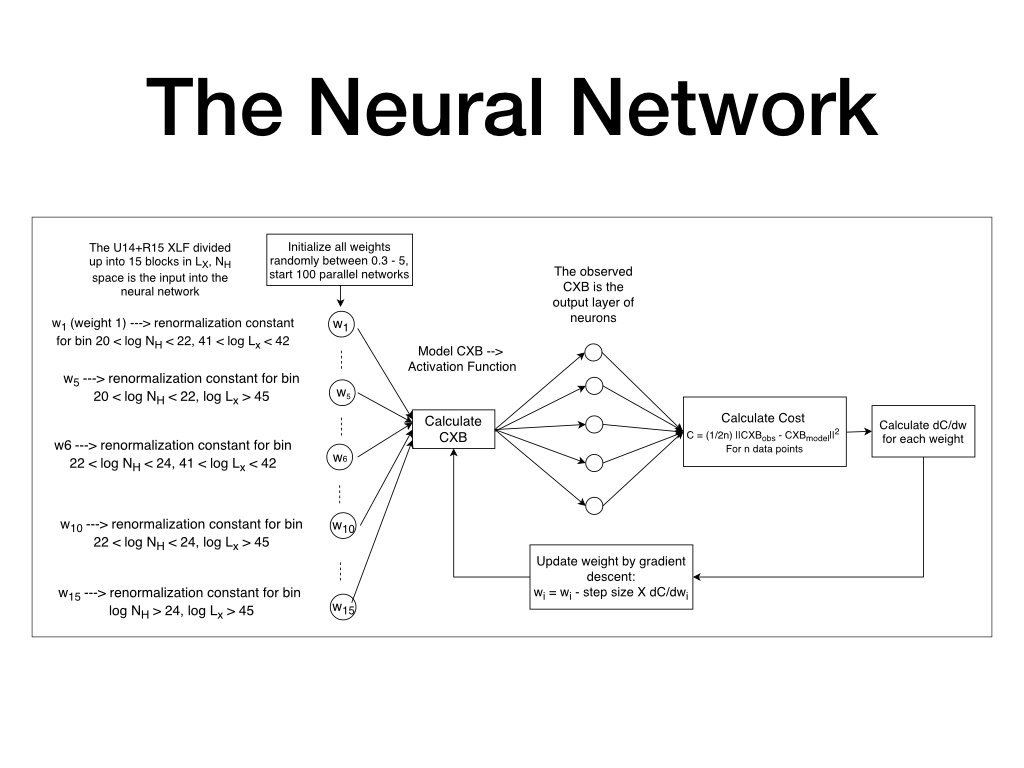
Neural Network to produce X-ray Luminosity Function
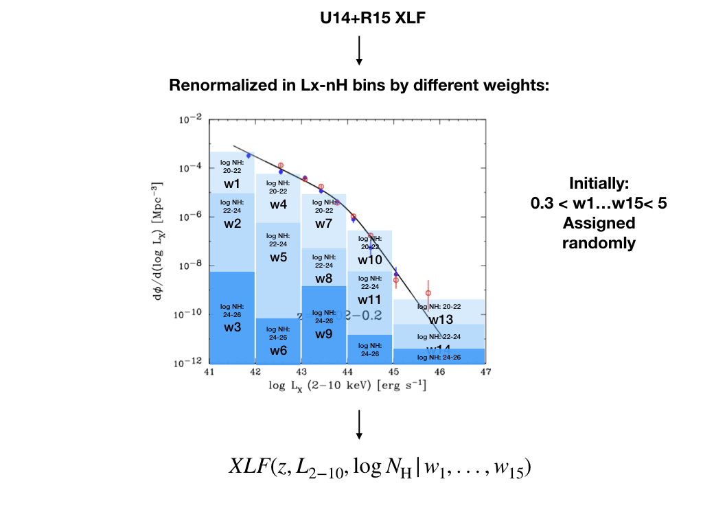
An X-ray population synthesis model describes the population of AGN at different epochs (z), at different Luminosity (Lx ) and obscuration levels (log NH). Paraphrasing, it answers the following question: how many AGN of luminosity Lx and column density log NH are there per unit comoving volume of the Universe at redshift z?
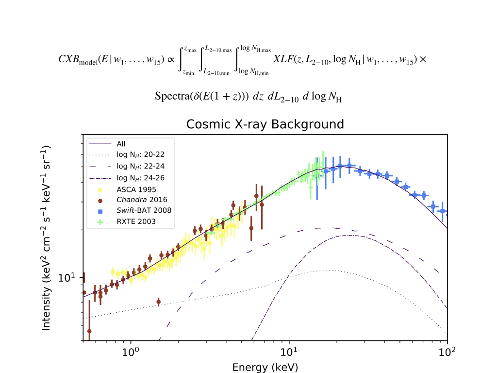
Using this underlying AGN population and assuming an AGN spectra, we can predict what the cosmic X-ray background (CXB) should look like, by performing the following calculation:

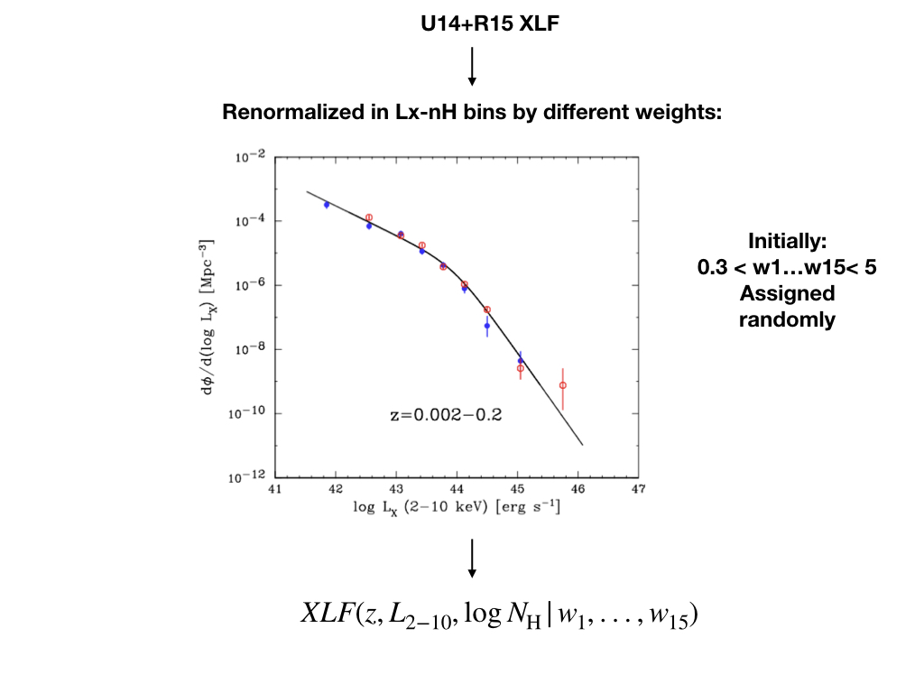
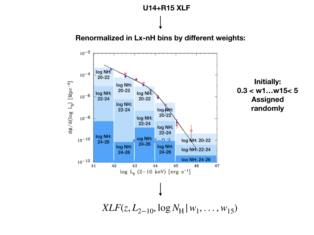
The image to the left is a typical XLF (from Ueda et. al. 2014) and the image to the right is a typical X-ray AGN spectra, and multiplying the number density with intensity of spectra at observed frame energy E, and integrating over all redshift, luminosities and obscuration levels produces the cosmic X-ray background.
X-ray surveys performed by XMM, Chandra, Swift-BAT and NuSTAR provide observed constraints such as number counts and Compton-thick fractions. These constraints, along with Cosmic X-ray background, must be satisfied by a correct underlying population/XLF.
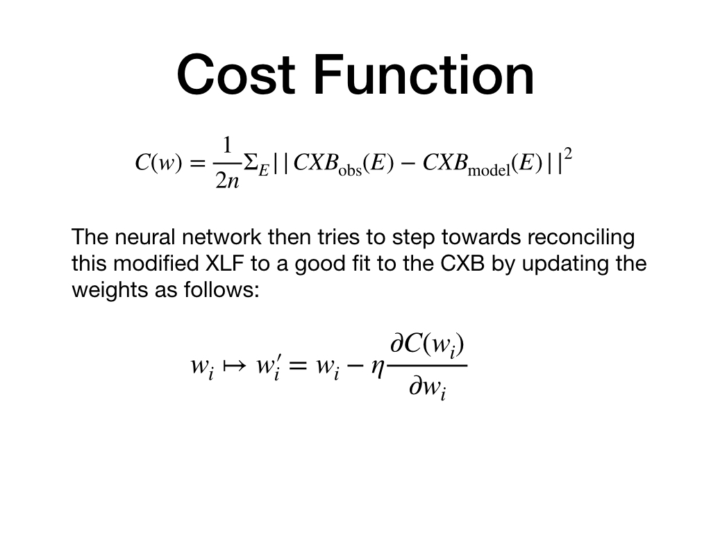
We constructed a neural network that produces a X-ray Luminosity Function which satisfies all the latest/most updated constraints from X-ray survey, which works as follows (click on the figure for more explanation):

Poster Presented at 17th HEAD Meeting related to this work can be found here.
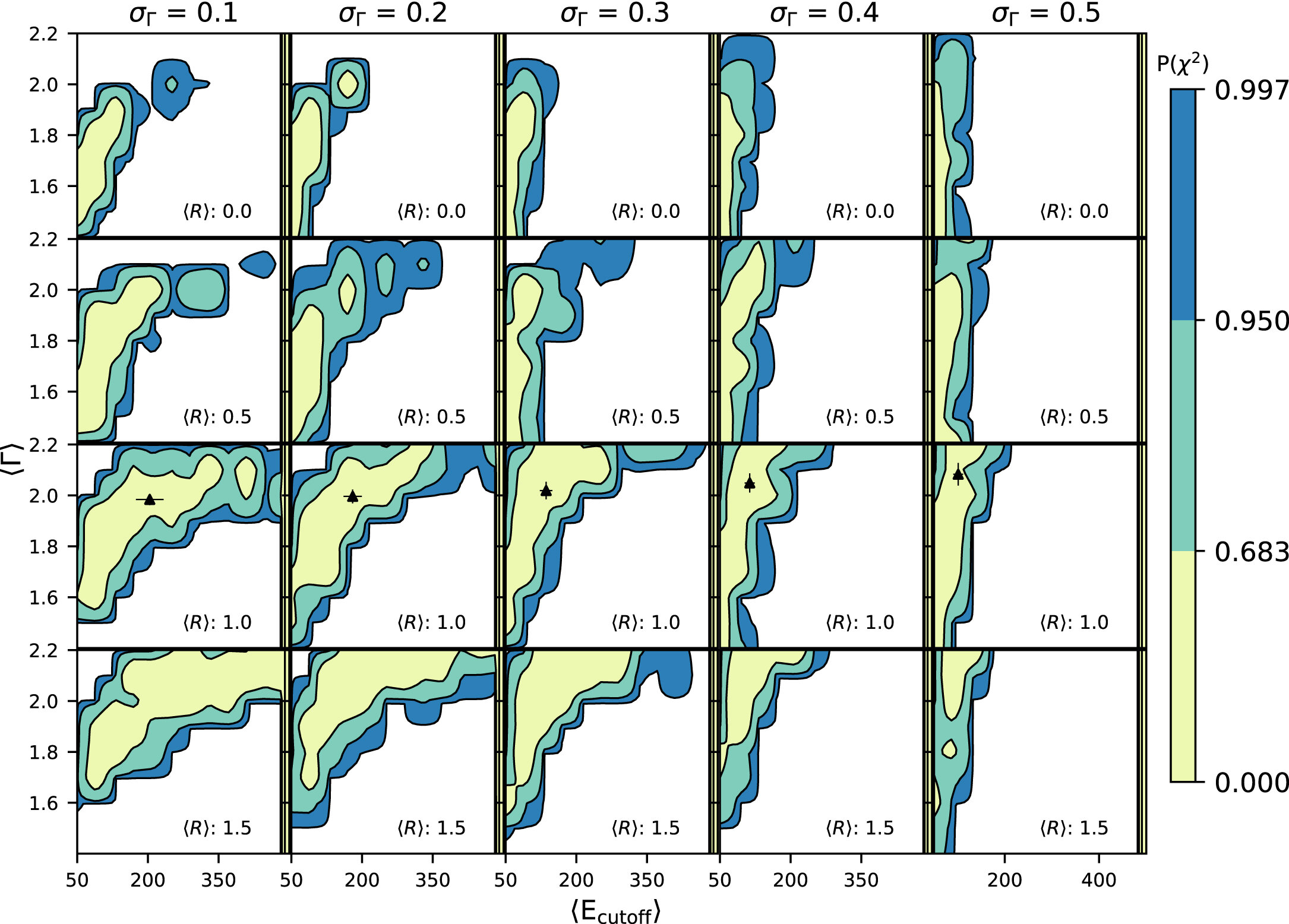
Allowed regions of the spectral parameter space, for unconstrained XLF. Contours for 1σ, 2σ and 3σ are shown in yellow, green, and blue, respectively. The black triangular data points indicate results of the Bayesian analysis using the XLF from Paper I. To create this figure, the same spectral set was assumed for all absorption bins. The values of σE and σR were kept constant at 36 keV and 0.14, respectively. The entire probability space can be explored quantitatively using the interactive tool described in Section 4.2, which allows users to specify a different spectral set for each absorption bin and explore other values of σE and σR as well as the variables shown in this plot.
Putting Strong Constraints on the AGN Spectral Parameter Space
We are only starting to constrain the AGN X-ray spectral parameter space observationally, but fitting AGN spectra is difficult due to biased samples (against obscured AGN and rare high luminosity AGN) and due to difficulties in constraining certain parameters. For example, high energy-cutoff of can only be constrained with NuSTAR or Swift-BAT data. which extends to very high energies).
A computational method of rejecting large parts of the AGN spectral parameter space is by using the shape of the Cosmic X-ray background (CXB). Under 100 keV, we expect most of the contribution to the cosmic X-ray background to come from AGN. X-ray population synthesis models focus on fitting the CXB using redshift, luminosity and obscuration dependent space densities of AGN. However, fitting the CXB is also dependent on the AGN spectra, and the parameter space of AGN spectra that can fit the CXB is limited. A comprehensive study using major X-ray spectral parameters (photon index, high energy cutoff and reflection scaling factor, and dispersions in each quantity) demonstrate these constraints.
This paper can be found here.
Photometric Redshifts and Population Types for ~6000 Stripe 82X objects
Stripe 82X is one of the largest volume X-ray surveys to date (31.3 square degrees). I calculated photometric redshifts for around 6000 X-ray selected objects in this region. These sources were mixed bag of both type 1 and type 2 AGNs, starburst galaxies, spirals, ellipticals and even some stars. Because these objects were not color selected to just be quasars, and because large volume X-ray surveys have different populations from smaller volume surveys, an had to construct an optimum set of templates that is small enough to avoid degeneracy in template SED-to-data fitting, and large enough to represent all the objects in the sample.
A big challenge in calculating photometric redshifts for large volume X-ray surveys is inhomogeneous data sets. Multi-wavelength photometry is needed to calculate photometric redshifts. For small X-ray surveys, this photometry is takes simultaneously and the images are registered to the same frame, so no positional cross-matching is necessary. However, for large volume X-ray surveys, multi-wavelength surveys with different depths and coverages, which are not registered positionally need to be compiled to produce SEDs. Here is an example we demonstrated in the paper:
Figure 3 from AGN Populations in Large-volume X-Ray Surveys: Photometric Redshifts and Population Types Found in the Stripe 82X Survey
Tonima Tasnim Ananna et al. 2017 ApJ 850 66 doi:10.3847/1538-4357/aa937d

Figure 3. From left to right: field of Stripe 82X XMM-Newton source ID 2794 (solid black circle with radius 7'') at the optical SDSS r band, near-infrared IRAC Ch1 (3.6 μm), and AllWISE W1 (3.4 μm). The positional errors for SDSS, VHS, and IRAC are only a few milliarcseconds; for clarity, we use bigger circles to indicate the location of the source in each band: a dashed green circle with radius 1'' around the SDSS r band, a solid yellow circle with radius 12 for the VHS K band, and a solid red circle with radius 1'' for the IRAC CH1 source positions. In this example, the most likely optical counterpart from the MLE analysis (left) is the bright source at the top (solid green circle), but the infrared images suggest a more reliable counterpart below and to the left. The dashed green circles indicate other nearby optical sources that have a lower reliability match. We identify the source circled in yellow as the correct counterpart, which is the most likely counterpart according to VHS and IRAC but more accurately pinpointed by VHS.
These figures show a 7" radius circle around the position of one X-ray source, as observed in SDSS r, IRAC CH1 and WISE W1 bands. This is a case where maximum likelihood match in different bands select different objects as the best match to the X-ray source. We created an extensive, reproducible pipeline to resolve conflicting associations:
Figure 6 from AGN Populations in Large-volume X-Ray Surveys: Photometric Redshifts and Population Types Found in the Stripe 82X Survey
Tonima Tasnim Ananna et al. 2017 ApJ 850 66 doi:10.3847/1538-4357/aa937d

Figure 6. Flow chart showing how we assign counterpart(s) to each X-ray source and how the QF is defined (see Section 2.5). QF values 1, 1.5, and 2 are secure; 3 and 4 are problematic; and −1 refers to the discarded, second-best candidate.
We were able to resolve these challenges and achieve accuracy comparable to smaller volume X-ray surveys with narrow and intermediate band photometry:

Figure 11. Spectroscopic vs. photometric redshift for point-like (left) and extended (right) sources in the uniform XMM-Newton fields. The results in the other fields are very similar, as can be seen in Table 7. Black crosses indicate cases where the primary redshift is incorrect and the secondary redshift is correct (i.e., it lies within the dashed black lines). The quantity "zphotN/A" reports the percentage of sources for which we are unable to calculate photometric redshifts altogether due to data in very few bands or not having an appropriate SED template in our template library.
Please contact me if you need help with such a pipeline, or need more information about the SED types used in this work, please consult the paper, or contact me!
Orion Nebula Treasury Program
I helped create an atlas for 8000 proto-stellar objects in the Orion Nebula, as part of the Hubble Telescope Orion Nebula Treasury Program. My contribution to this project involved making image cutouts from Hubble Space Telescope’s ACS, NICMOS and WFPC2 images, as well as some ground based observations (WFI and ISPI), and compiling them in one catalog containing these images as well as the calculated magnitudes.
The data products are available here.
Credit for top template image of Carina Nebula: NASA/STScI